import numpy as np
import pandas as pd
import matplotlib.pyplot as plt
import seaborn as sns
import geopandas as gpd
import contextily as ctxAppendix A — Appendix for Chapter 14
A.1 The California School Districts Dataset
In this section, we first generate a map showing the geographical boundaries of all school districts in California. We then provide choropleth maps illustrating how various characteristics are distributed across these districts.
Recall that our dataset in the caschool.csv file contains information on kindergarten through eighth-grade students across 420 California school districts (K-6 and K-8 districts) in 1999. The column names are given below:
# Column names
CAschool=pd.read_csv('data/caschool.csv')
CAschool.columns
Index(['Observation Number', 'dist_cod', 'county', 'district', 'gr_span',
'enrl_tot', 'teachers', 'calw_pct', 'meal_pct', 'computer', 'testscr',
'comp_stu', 'expn_stu', 'str', 'avginc', 'el_pct', 'read_scr',
'math_scr'],
dtype='object')To map the school districts, we use the shapefile California_School_District_Areas_2024-25.shp, obtained from the California Department of Education website. This shapefile contains geographical boundaries for all school districts in California for the 2024-25 academic year.
# Load shapefile
gdf = gpd.read_file("data/California_School_District_Areas_2024-25.shp")
gdf.columns
Index(['OBJECTID', 'Year', 'FedID', 'CDCode', 'CDSCode', 'CountyName',
'DistrictNa', 'DistrictTy', 'GradeLow', 'GradeHigh', 'GradeLowCe',
'GradeHighC', 'AssistStat', 'CongressUS', 'SenateCA', 'AssemblyCA',
'UpdateNote', 'EnrollTota', 'EnrollChar', 'EnrollNonC', 'AAcount',
'AApct', 'AIcount', 'AIpct', 'AScount', 'ASpct', 'FIcount', 'FIpct',
'HIcount', 'HIpct', 'PIcount', 'PIpct', 'WHcount', 'WHpct', 'MRcount',
'MRpct', 'NRcount', 'NRpct', 'ELcount', 'ELpct', 'FOScount', 'FOSpct',
'HOMcount', 'HOMpct', 'MIGcount', 'MIGpct', 'SWDcount', 'SWDpct',
'SEDcount', 'SEDpct', 'DistrctAre', 'Shape__Are', 'Shape__Len',
'geometry'],
dtype='object')In the following map, we show the geographical boundaries of all school districts in California. We use the contextily package to add a basemap to the plot.
# Plotting with basemap
gdf = gdf.to_crs(epsg=3857)
ax = gdf.plot(
    figsize=(10,10),
    edgecolor="white",
    linewidth=0.5
)
ctx.add_basemap(ax)
ax.axis('off')
plt.show()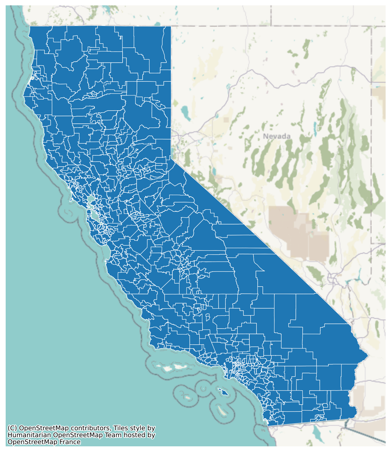
The total number of school districts in the shapefile is given by:
# Number of school districts in shapefile
len(gdf)937However, not all school districts in the shapefile are present in the caschool.csv dataset. To identify the school districts common to both datasets, we perform an inner merge based on the district codes. The dist_cod column in caschool.csv represents the unique identifier for each school district, while in the shapefile the corresponding column is CDCode (the last five digits). We use these columns to merge our dataset with the gdf dataframe.
# Take last five digits of district CDCode in shapefile
gdf["CDCode_str"] = gdf["CDCode"].astype(str).str[-5:]
# Make district code in data string
CAschool["dist_cod_str"] = CAschool["dist_cod"].astype(str)
# Merge data with shapefile
merged_gdf = gdf.merge(CAschool, left_on="CDCode_str", right_on="dist_cod_str", how="left")
In the next figure, we create choropleth maps to show how variables of interest are distributed across California school districts. We consider the average test scores (testscr), the student-teacher ratio (str), the average district income (avginc), and the percentage of English learners (el_pct) in the districts.
# Choropleth Maps of School District Characteristics
fig, axs = plt.subplots(2, 2, figsize=(10, 12))
# Test Scores
merged_gdf.plot(column="testscr", ax=axs[0, 0], cmap="viridis",
              legend=True,
              legend_kwds={
                "shrink": 0.5,
                "aspect": 20,
                "pad": 0.02,
                "orientation": "horizontal"
              })
axs[0, 0].set_title("Test Scores", fontsize=10)
axs[0, 0].axis('off')
# Student-Teacher Ratio
merged_gdf.plot(column="str", ax=axs[0, 1], cmap="viridis",
              legend=True,
              legend_kwds={
                "shrink": 0.5,
                "aspect": 20,
                "pad": 0.02,
                "orientation": "horizontal"
              })
axs[0, 1].set_title("Student-Teacher Ratio", fontsize=10)
axs[0, 1].axis('off')
# Average Income
merged_gdf.plot(column="avginc", ax=axs[1, 0], cmap="viridis",
              legend=True,
              legend_kwds={
                "shrink": 0.5,
                "aspect": 20,
                "pad": 0.02,
                "orientation": "horizontal"
              })
axs[1, 0].set_title("Average Income", fontsize=10)
axs[1, 0].axis('off')
# English Learner Percentage
merged_gdf.plot(column="el_pct", ax=axs[1, 1], cmap="viridis",
              legend=True,
              legend_kwds={
                "shrink": 0.5,
                "aspect": 20,
                "pad": 0.02,
                "orientation": "horizontal"
              })
axs[1, 1].set_title("English Learner Percentage", fontsize=10)
axs[1, 1].axis('off')
plt.show()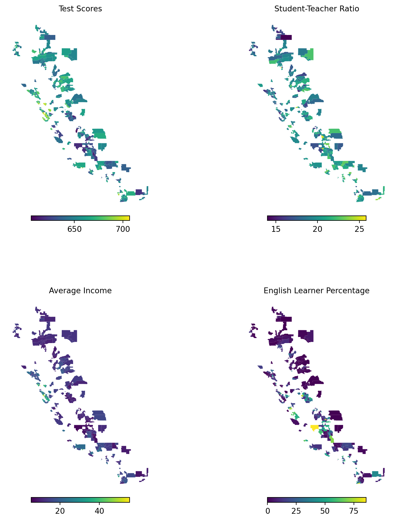
Finally, we create choropleth maps for the percentage of students eligible for free or reduced-price lunch (meal_pct) and the percentage of students receiving CalWORKs assistance (calw_pct).
# Choropleth Maps of Assistance Programs
# Meal Percentage
fig, axs = plt.subplots(1, 2, figsize=(10, 6))
merged_gdf.plot(column="meal_pct", ax=axs[0], cmap="viridis",
              legend=True,
              legend_kwds={
                "shrink": 0.5,
                "aspect": 20,
                "pad": 0.02,
                "orientation": "horizontal"
              })
axs[0].set_title("Reduced-Price Lunch Percentage", fontsize=10)
axs[0].axis('off')
# CalWORKs Assistance Percentage
merged_gdf.plot(column="calw_pct", ax=axs[1], cmap="viridis",
              legend=True,
              legend_kwds={
                "shrink": 0.5,
                "aspect": 20,
                "pad": 0.02,
                "orientation": "horizontal"
              })
axs[1].set_title("CalWORKs Assistance Percentage", fontsize=10)
axs[1].axis('off')
plt.show()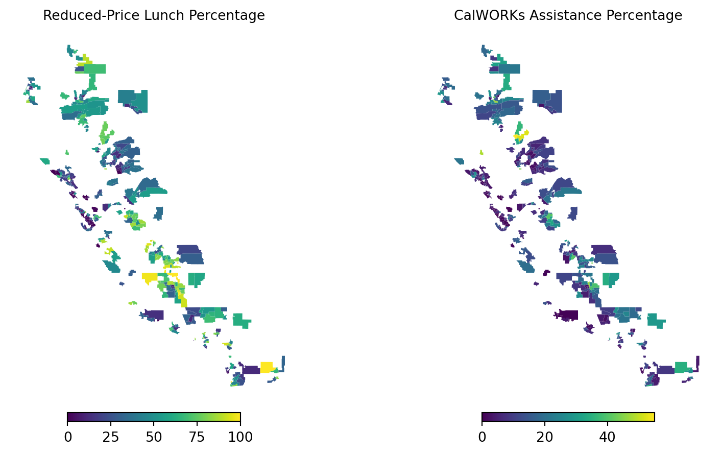
A.2 Derivation of the OLS estimators
Consider a linear regression model with an intercept and only one explanatory variable: \[ Y_i=\beta_0+\beta_1 X_i+ u_i, \] for \(i=1,\dots,n\). In this section, we derive the following OLS estimators: \[ \begin{align} &\hat{\beta}_1=\frac{\sum_{i=1}^n\big(X_i-\bar{X}\big)\big(Y_i-\bar{Y}\big)}{\sum_{i=1}^n\big(X_i-\bar{X}\big)^2} \quad\text{and}\quad \hat{\beta}_0=\bar{Y}-\hat{\beta}_1\bar{X}, \end{align} \tag{A.1}\] where \(\bar{Y}=\frac{1}{n}\sum_{i=1}^nY_i\) and \(\bar{X}=\frac{1}{n}\sum_{i=1}^nX_i\).
The least-squares estimators are defined as \[ \begin{align} (\hat{\beta}_0,\,\hat{\beta}_1)^{'}&=\argmin_{\beta_0,\,\beta_1}\sum_{i=1}^n\big(Y_i-\beta_0-\beta_1X_i\big)^2. \end{align} \] We set the first-order conditions of the objective function with respect to \(\beta_0\) and \(\beta_1\) equal to zero: \[ \begin{align*} \frac{\partial \sum_{i=1}^n\big(Y_i-\beta_0-\beta_1X_i\big)^2}{\partial\beta_0}&=-2\sum_{i=1}^n\big(Y_i-\beta_0-\beta_1X_i\big)=0,\\ \frac{\partial \sum_{i=1}^n\big(Y_i-\beta_0-\beta_1X_i\big)^2}{\partial\beta_1}&=-2\sum_{i=1}^nX_i\big(Y_i-\beta_0-\beta_1X_i\big)=0. \end{align*} \]
From the first equation, we can solve for \(\beta_0\) as \[ \begin{align*} &-2\sum_{i=1}^n\big(Y_i-\beta_0-\beta_1X_i\big)=0\implies \sum_{i=1}^n\big(Y_i-\beta_0-\beta_1X_i\big)=0,\\ &\implies \sum_{i=1}^n\big(Y_i-\beta_1X_i\big)-\sum_{i=1}^n\beta_0=0\implies \sum_{i=1}^n\big(Y_i-\beta_1X_i\big)=n\beta_0. \end{align*} \] Thus, the solution for \(\beta_0\) yields \[ \begin{align*} \hat{\beta}_0=\frac{1}{n}\sum_{i=1}^n\big(Y_i-\beta_1X_i\big)=\frac{1}{n}\sum_{i=1}^nY_i -\beta_1\frac{1}{n}\sum_{i=1}^nX_i=\bar{Y}-\beta_1\bar{X}. \end{align*} \]
Substituting the solution for \(\beta_0\) into the second equation yields \[ \begin{align*} &-2\sum_{i=1}^nX_i\big(Y_i-[\bar{Y}-\beta_1\bar{X}]-\beta_1X_i\big)=0\implies\sum_{i=1}^nX_i\big(Y_i-[\bar{Y}-\beta_1\bar{X}]-\beta_1X_i\big)=0\\ &\implies\sum_{i=1}^nX_i\big(Y_i-\bar{Y})-\beta_1\sum_{i=1}^nX_i\big(X_i-\bar{X}\big)=0. \end{align*} \]
Hence, solution for \(\beta_1\) is \[ \begin{align} \hat{\beta}_1=\frac{\sum_{i=1}^nX_i\big(Y_i-\bar{Y})}{\sum_{i=1}^nX_i\big(X_i-\bar{X}\big)}. \end{align} \tag{A.2}\]
The numerator \(\sum_{i=1}^nX_i\big(Y_i-\bar{Y})\) can be expressed as \(\sum_{i=1}^n\big(X_i-\bar{X}\big)\big(Y_i-\bar{Y}\big)\), because \[ \begin{align*} \sum_{i=1}^nX_i\big(Y_i-\bar{Y})&=\sum_{i=1}^nX_iY_i-\sum_{i=1}^nX_i\bar{Y}=\sum_{i=1}^nX_iY_i-\bar{Y}\sum_{i=1}^nX_i-n\bar{X}\bar{Y}+n\bar{X}\bar{Y}\\ &=\sum_{i=1}^nX_iY_i-\bar{Y}\sum_{i=1}^nX_i-\bar{X}\sum_{i=1}^nY_i+n\bar{X}\bar{Y}\\ &=\sum_{i=1}^nX_iY_i-\bar{Y}\sum_{i=1}^nX_i-\bar{X}\sum_{i=1}^nY_i+\sum_{i=1}^n\bar{X}\bar{Y}\\ &=\sum_{i=1}^n\big(X_iY_i-\bar{Y}X_i-\bar{X}Y_i+\bar{X}\bar{Y}\big)=\sum_{i=1}^n\big(X_i-\bar{X}\big)\big(Y_i-\bar{Y}\big). \end{align*} \]
Similarly, the denominator of \(\hat{\beta}_1\) can be expressed as \[ \begin{align*} &\sum_{i=1}^nX_i\big(X_i-\bar{X}\big)=\sum_{i=1}^nX_i^2-\sum_{i=1}^nX_i\bar{X}=\sum_{i=1}^nX_i^2-\sum_{i=1}^nX_i\bar{X}-n\bar{X}^2+n\bar{X}^2\\ &=\sum_{i=1}^nX_i^2-\bar{X}\sum_{i=1}^nX_i-\sum_{i=1}^n\bar{X}\bar{X}+\sum_{i=1}^n\bar{X}^2=\sum_{i=1}^nX_i^2-\bar{X}\sum_{i=1}^nX_i-\bar{X}\sum_{i=1}^nX_i+\sum_{i=1}^n\bar{X}^2\\ &=\sum_{i=1}^n\big(X_i^2-2\bar{X}X_i+\bar{X}^2\big)=\sum_{i=1}^n\big(X_i-\bar{X}\big)^2. \end{align*} \]
Thus, Equation A.2 is equivalent to Equation A.1. Finally, we can substitute \(\hat{\beta}_1\) back to \(\hat{\beta}_0\) to obtain the solution for \(\beta_0\): \[ \begin{align*} \hat{\beta}_0=\bar{Y}-\hat{\beta}_1\bar{X}. \end{align*} \]
A.3 Algebraic properties of the OLS estimators
We show that the least squares residuals sum to zero, i.e., \(\sum_{i=1}^n\hat{u}_i=0\). Using \(\hat{u}_i=(Y_i-\hat{\beta}_0-\hat{\beta}_1X_i)\), we have \[ \begin{align*} \sum_{i=1}^n\hat{u}_i &=\sum_{i=1}^n\big(Y_i-\hat{\beta}_0-\hat{\beta}_1X_i\big)=\sum_{i=1}^n\big(Y_i-[\bar{Y}-\hat{\beta}_1\bar{X}]-\hat{\beta}_1X_i\big)\\ &=\sum_{i=1}^n\big(Y_i-\bar{Y}\big)-\hat{\beta}_1\sum_{i=1}^n\big(X_i-\bar{X}\big)\\ &=\sum_{i=1}^n\big(Y_i-\bar{Y}\big)-\left(\frac{\sum_{i=1}^nX_i\big(Y_i-\bar{Y})}{\sum_{i=1}^nX_i\big(X_i-\bar{X}\big)}\right)\sum_{i=1}^n\big(X_i-\bar{X}\big)=0, \end{align*} \] because \(\sum_{i=1}^n\big(Y_i-\bar{Y}\big)=\sum_{i=1}^nY_i-\sum_{i=1}^n\bar{Y}=n\bar{Y}-n\bar{Y}=0\) and \(\sum_{i=1}^n\big(X_i-\bar{X}\big)=\sum_{i=1}^nX_i-\sum_{i=1}^n\bar{X}=n\bar{X}-n\bar{X}=0\).
Next, we show that the correlation between residuals and regressors is zero, i.e., \(\sum_{i=1}^nX_i\hat{u}_i=0\). Using \(\hat{u}_i=(Y_i-\hat{\beta}_0-\hat{\beta}_1X_i)\), we obtain \[ \begin{align*} \sum_{i=1}^nX_i\hat{u}_i &=\sum_{i=1}^nX_i\big(Y_i-\hat{\beta}_0-\hat{\beta}_1X_i\big)=\sum_{i=1}^nX_i\big(Y_i-[\bar{Y}-\hat{\beta}_1\bar{X}]-\hat{\beta}_1X_i\big)\\ &=\sum_{i=1}^nX_i\big(Y_i-\bar{Y}\big)-\hat{\beta}_1\sum_{i=1}^nX_i\big(X_i-\bar{X}\big)\\ &=\sum_{i=1}^nX_i\big(Y_i-\bar{Y}\big)-\left(\frac{\sum_{i=1}^nX_i\big(Y_i-\bar{Y})}{\sum_{i=1}^nX_i\big(X_i-\bar{X}\big)}\right)\sum_{i=1}^nX_i\big(X_i-\bar{X}\big)\\ &=\sum_{i=1}^nX_i\big(Y_i-\bar{Y}\big)-\sum_{i=1}^nX_i\big(Y_i-\bar{Y}\big)=0. \end{align*} \]
Finally, we show that the regression line passes through the sample mean, i.e., \(\bar{Y}=\hat{\beta}_0+\hat{\beta}_1\bar{X}=\bar{\hat{Y}}\). Using
\(Y_i=(\hat{Y}_i+\hat{u}_i)\) and \(\hat{Y}_i=(\hat{\beta}_0+\hat{\beta}_1X_i)\), we obtain
\[ \begin{align*} \bar{Y}&=\frac{1}{n}\sum_{i=1}^nY_i=\frac{1}{n}\sum_{i=1}^n(\hat{Y}_i+\hat{u}_i)=\frac{1}{n}\sum_{i=1}^n\hat{Y}_i +\frac{1}{n}\sum_{i=1}^n\hat{u}_i\\ &=\frac{1}{n}\sum_{i=1}^n(\hat{\beta}_0+\hat{\beta}_1X_i) +\frac{1}{n}\sum_{i=1}^n\hat{u}_i =\frac{1}{n}\sum_{i=1}^n\hat{\beta}_0+\frac{1}{n}\sum_{i=1}^n\hat{\beta}_1X_i +\frac{1}{n}\sum_{i=1}^n\hat{u}_i\\ &=\frac{1}{n}\sum_{i=1}^n\hat{\beta}_0+\hat{\beta}_1\frac{1}{n}\sum_{i=1}^nX_i +\frac{1}{n}\sum_{i=1}^n\hat{u}_i =\hat{\beta}_0+\hat{\beta}_1\bar{X}+0\\ &=\hat{\beta}_0+\hat{\beta}_1\bar{X}. \end{align*} \]